Manufacturing Loss Data Visualizer & Analyzer
Drop in an Excel file, get a dashboard you can drill into
Background & Problem
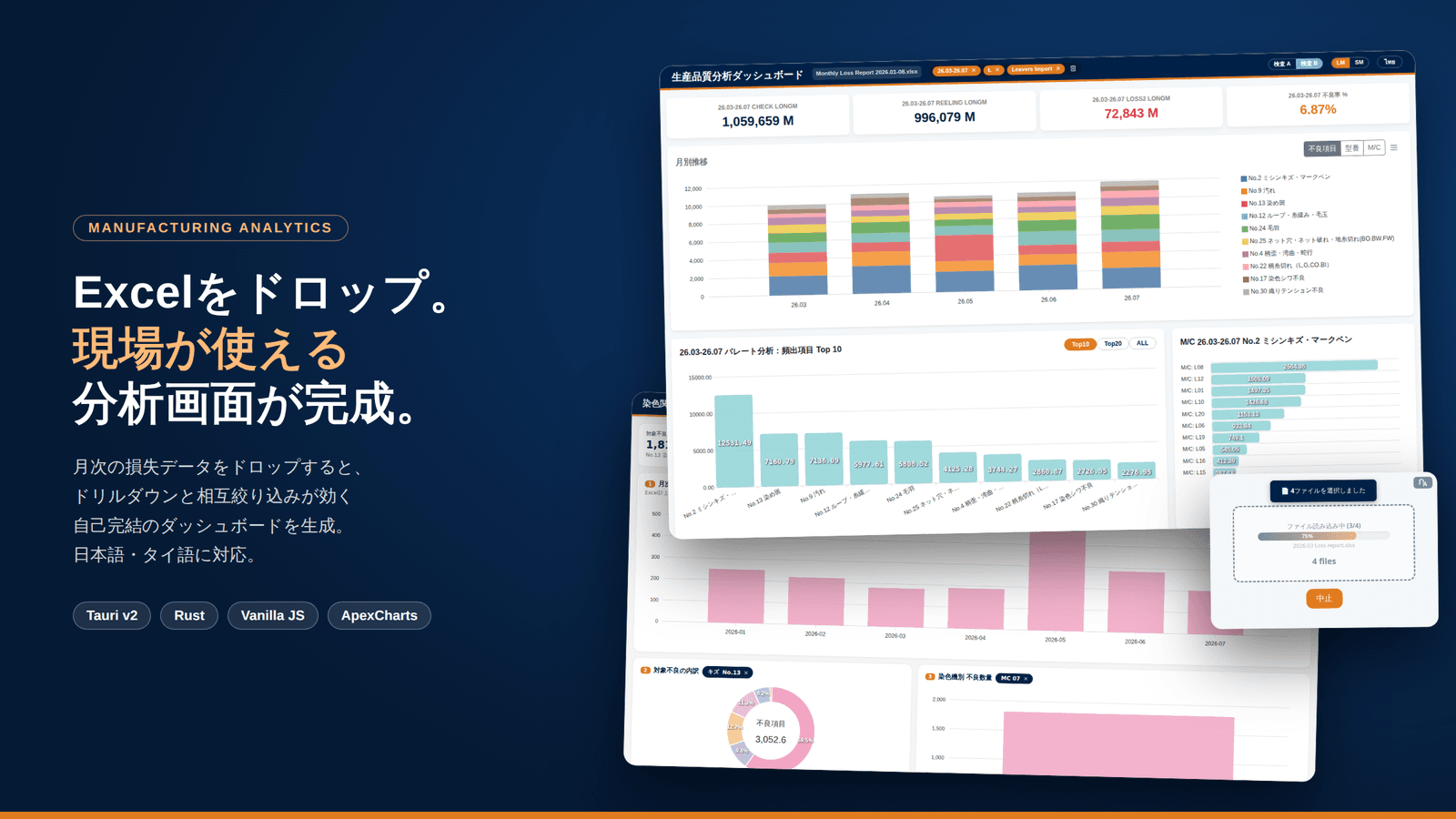
In manufacturing, monthly loss data accumulates in one Excel workbook at the granularity of process, machine type, model number and production lot. Each file holds several sheets of multiple megabytes, and answering 'which defect is high, on which model, on which machine?' meant re-filtering and tallying by hand. The people reading the result range from floor staff to managers, and some sites are Thai-speaking. When only the analyst holds the numbers, the improvement discussion never starts. The goal was a report anyone could open without a special environment and drill into on the spot.
Key Features
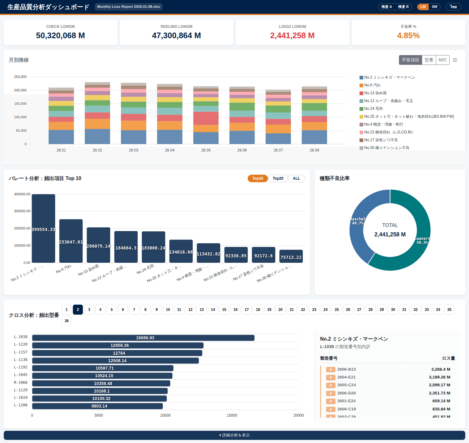
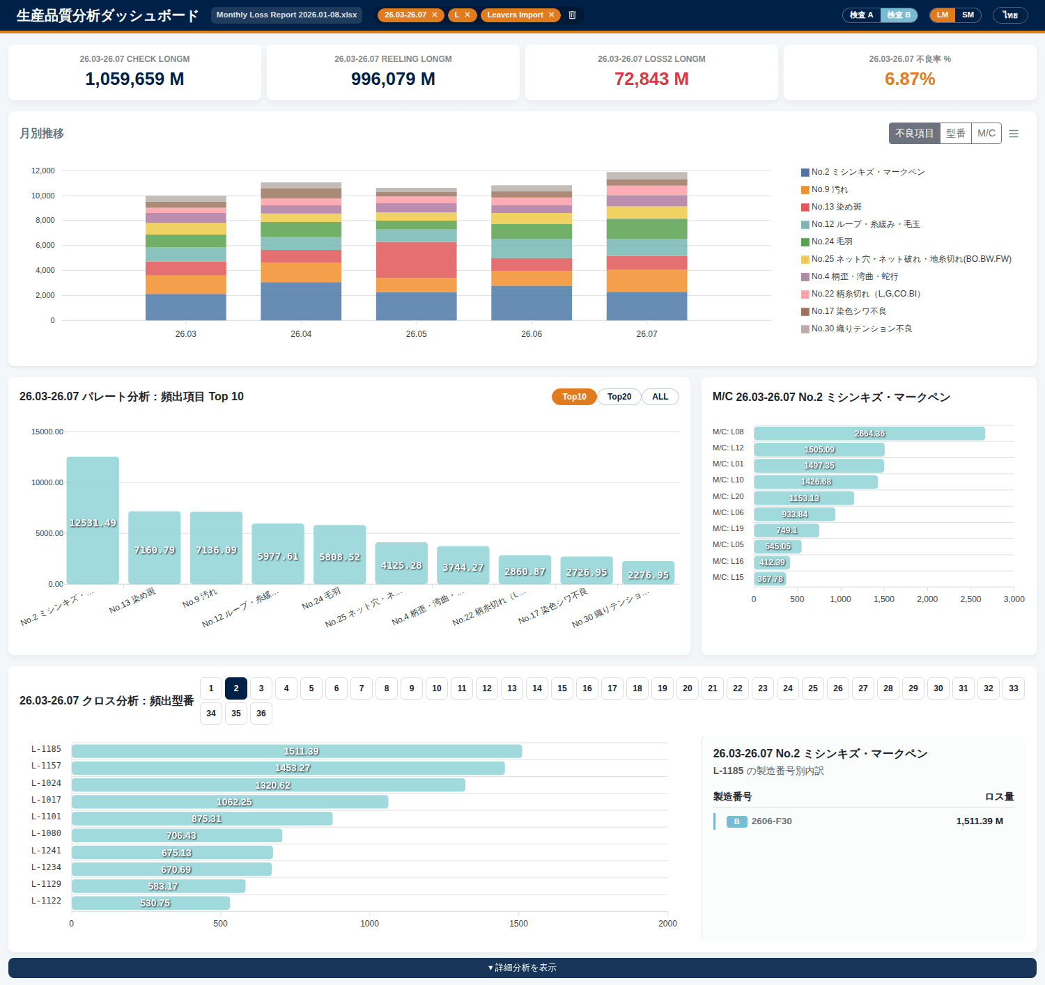
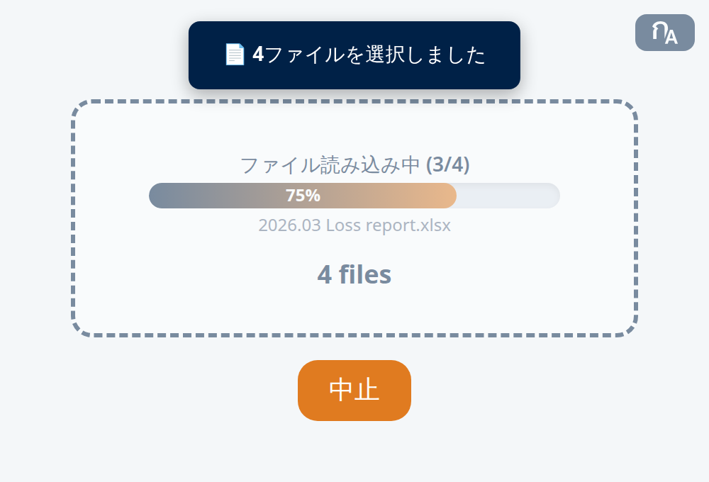
Drop several Excel files and the app generates a single dashboard: a Pareto chart of defects, a monthly trend, and cross analysis by machine and model. Every chart is linked; clicking the donut centre steps back one level, and dragging the monthly chart zooms the period. Active filters are always visible as chips at the top and can be cleared one by one. Machine type and in-house/outsourced are drilled through a two-level donut. The inspection site, by contrast, is an independent axis placed in the navigation bar as a toggle, so it applies to every chart in one click at any depth. I kept it out of the hierarchy so that an axis that should always be visible as a KPI is not hidden three clicks deep. Japanese and Thai switch with a single button that shows the language you will switch to.
Technical Approach & Architecture
Three reasons for Tauri v2 + Rust. (1) Sheet XML in these workbooks reaches several MB, so batch aggregation across files suits native code. (2) It runs on internal PCs and should complete locally without standing up a server. (3) The distributable should stay small (the release build is configured for size and LTO). The output is a self-contained HTML file with data and logic embedded. Viewers do not need the app; sending the file by email or chat is enough. One honest limitation: the chart library and fonts are still loaded from a CDN, so viewing currently needs network access. Fully offline output (inlining them) remains on the improvement list.
Engineering Highlight 1: Reading the inspection site from cell formatting
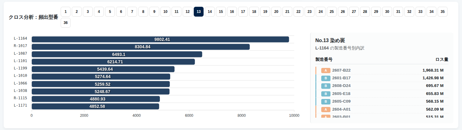
The business rule is that a filled background in the month column means the row was inspected at one site, and no fill means the other. But the Excel-reading crate in use (calamine) returns only cell values, not fill colours. I compared a fork that reads styles, another full-featured crate, a port of Python's openpyxl, and SheetJS. The fork carries maintenance risk, the full-featured crate means carrying a second complete parser with row-alignment risk, and SheetJS reads fill colours only in its paid edition. Instead, I used the fact that xlsx is a ZIP and read only the style definitions and the target column's cells: cell style index, then cell format, then fill definition. The only additions are a lightweight ZIP crate and regex. Before implementing, I checked the colour distribution on 19 real files (about 40k rows) and reproduced the same procedure in Python to confirm the results matched. Each web row in the detail panel now carries an inspection-site tag, and every chart can be filtered by site.
Engineering Highlight 2: No silent failures
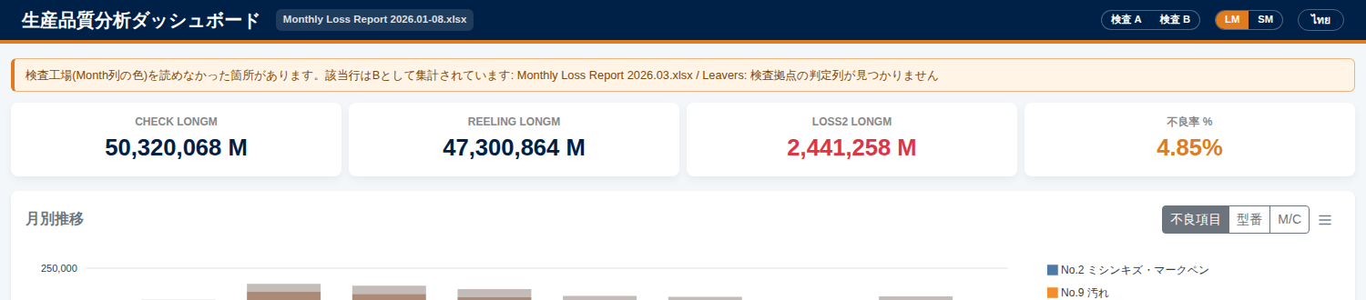
If the colour cannot be read, every row falls on the 'no fill' side. At first I swallowed the failure and kept aggregating, but once the inspection site became part of the bucket key, a failure could distort the aggregate itself. Files and sheets that could not be read are now collected and shown as a warning banner at the top of the report. The second was my own configuration mistake. I added the ZIP crate with default features, and a real-machine cargo check showed 22 extra packages in the lockfile, including crates that need a C compiler. Only deflate is needed for xlsx, so I disabled the defaults and confirmed the 22 packages disappeared from the lockfile. Also, loosening sheet-name matching to absorb variations (trailing spaces, case) started to pick up sheets in a different layout, so those are now excluded by name.
Engineering Highlight 3: Data design for size and speed
All numbers are recomputed in the browser, so monthly data is embedded as-is. Keys are shortened, all-period and all-department totals are not emitted but derived from monthly data in the browser, and department buckets are computed lazily on first access, which keeps the HTML light. Adding the inspection site raises the department keys from four to eight, so I estimated the growth on 19 real files first. The row data that dominates the size is only redistributed (0.0% growth), model-number keys grew about 24%, and machine keys about 64%. Not emitting empty buckets offsets part of that increase.
Executive-level Analysis
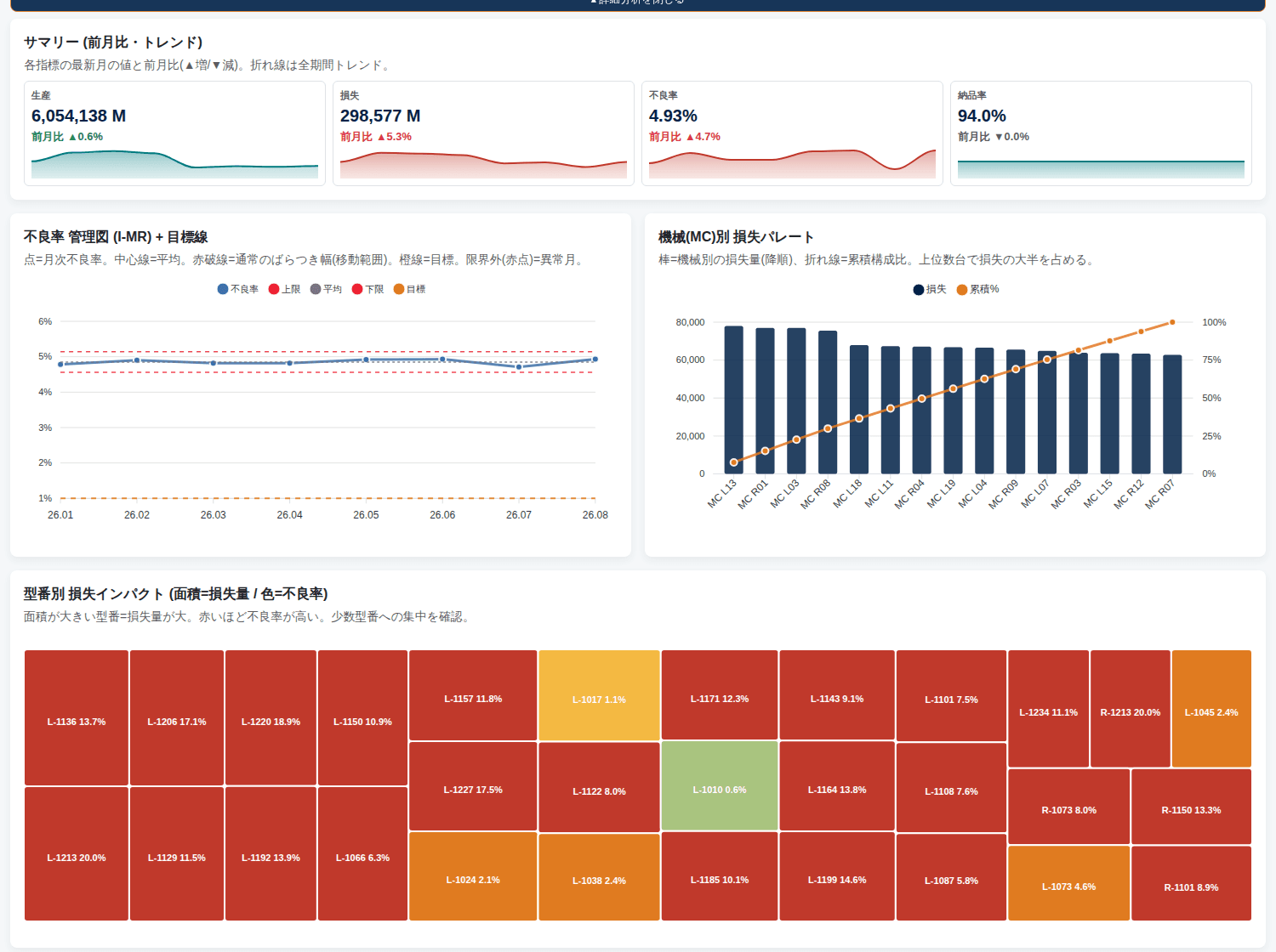
For multi-month reports there is a collapsible advanced section: KPI summary with month-over-month change, a control chart of defect rate (individuals and moving range), a Pareto chart of loss by machine with cumulative ratio, and a treemap of loss impact by model. Each comes with a plain-language 'how to read' note so the numbers can be interpreted without explanation.
Bilingual Support
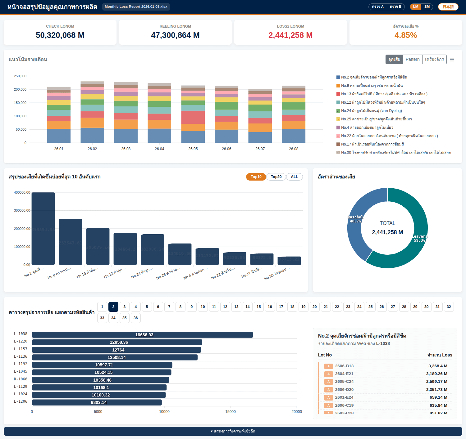
The whole screen, chart legends and defect names switch between Japanese and Thai to match the site staff. Because word order differs between the two languages, dynamic phrases such as 'Top N' in headings are templates with a number placeholder so that each language reads naturally.
Companion App: Dyeing defect analysis joined with the production database
The loss Excel records defects but not which dyeing machine processed the lot. I built a separate app that joins the loss Excel with dyeing-plan records in the production database directly over ODBC. The join key is model number plus lot number (zero-padded to six digits); because lot numbers cycle yearly, I take the dyeing date closest to the Excel year and month. The machine identification rate on real data is about 97%. Unmatched rows are kept as 'unknown' so the defect totals still equal the source data (0.0% difference from the reference data). The main cause of non-matches is lot numbers that differ between the Excel and the DB for the same model; a fallback join on model number plus date proximity is the next improvement under consideration.
Cross-filtering toward the cause
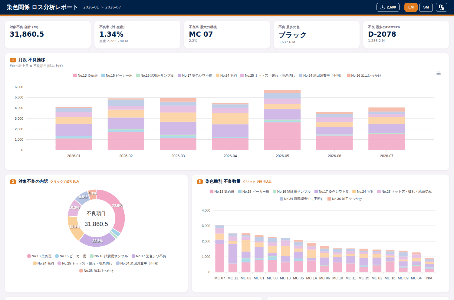
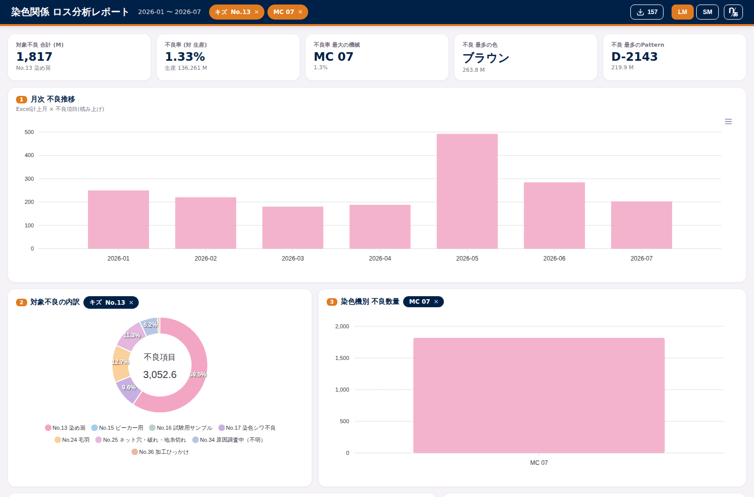
All charts and tables recompute under conditions such as defect type, machine, model number, colour, re-dyeing, weekday, bath count and dyeing count. The image shows the report filtered to one defect and then to one machine, and the monthly trend reveals a month where that defect spiked. The filtered result can be listed as detail rows and exported to CSV.
Statistics to separate noise from anomalies
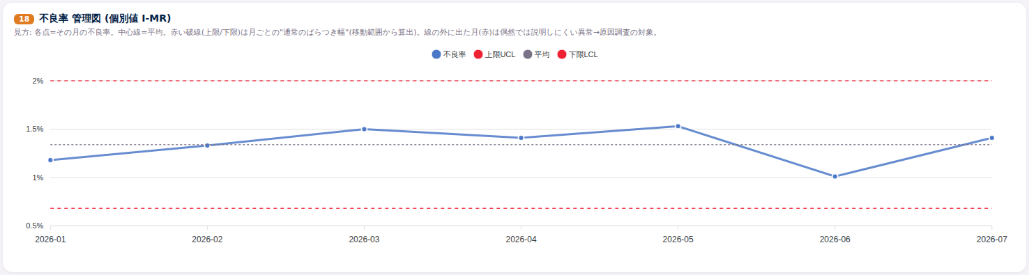
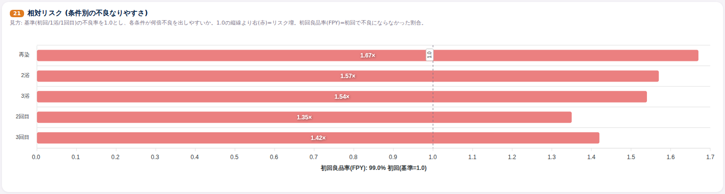
Monthly defect rate is judged with an individuals/moving-range control chart (mean plus or minus 2.66 times the average moving range). I first considered a p-chart, but production volume is large and the data is overdispersed, so I switched to the individuals method. Machine-by-defect skew is shown as a heatmap of standardised residuals that corrects for differences in volume, and conditions such as first-pass versus re-dyed or bath count are shown as relative risk against a baseline of 1.0. A co-occurrence matrix of rows with several defects at once helps look for common causes. Each card includes a 'how to read' note.
Machine-by-defect skew at a glance
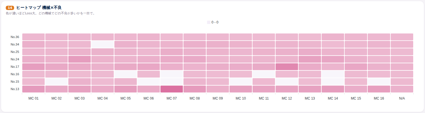
A heatmap shows loss by machine and defect. Machines where dark cells concentrate are the first candidates for investigation. Used with the Pareto chart of loss by machine and its cumulative ratio, it also shows how concentrated the loss is in a few machines.
Is re-dyeing really more defect-prone?
The first pass, single bath and first dyeing are the baseline (1.0), and each condition is shown as a multiple of the baseline defect rate, together with the first-pass yield. The feeling that re-dyeing seems to produce more defects can be checked as numbers by condition.
Outcome, Current State & What Is Next
Using the existing Excel as-is, the tools now generate analysis screens that take a reader from the overall picture to the cause without re-tallying in a spreadsheet. Bilingual support, inspection-site filtering, machine identification through the production database and statistical analysis are all implemented across the two apps and being refined on real machines. Quantified outcomes such as hours saved are 'to be confirmed' because no before-and-after measurement was taken. Open items are fully offline output (inlining the chart library), the database-join fallback, and converting loss into monetary terms (unit prices not yet provided), all ongoing. Part of the development happened without a Windows machine, so Rust-side changes are built and verified on a real machine step by step.